
- AdaptWest |
- Land Facet Data for North America
Land Facet Data for North America
The datasets below provide information on the physical habitat or land facet types of North America at 100m resolution.
Download links are at the bottom of this page.
For a document containing further information on the dataset see:
LAND FACETS AS A CONSERVATION TARGET IN CONSERVATION PLANNING FOR CLIMATE ADAPTATION
One potential strategy for protecting biodiversity in a changing climate is based on the idea of protecting the diversity of abiotic conditions that influence patterns of biodiversity. In this strategy, conservation features (the “targets” considered in the conservation planning process) are derived from data on physical features such as topography, soils, and geology. This approach is fundamentally a “coarse-filter” representation strategy based on physical habitat types. The approach has also been described as “conserving the ecological stage” or protecting “land facets” or “enduring features” (see this recent Special Section in the journal Conservation Biology for more background).
Species distributions,
communities, ecosystems, and broader patterns of biodiversity are clearly
influenced by abiotic drivers such as soils, geology, topography, and climate. Although
climates will change relatively rapidly over the coming century, soils,
geology, and topography will not. Thus, local, and some regional, climate
patterns and gradients influenced by topography will persist (e.g., higher
elevations will still be cooler than lower elevations, although both will likely
be warmer) as climates change. The hypothesis underlying use of land facets in
climate adaptation planning is that by protecting a diversity of land facets,
it may be possible to protect areas that will foster a diversity of biota in
the future, albeit different biota than those areas would protect today. Although
land facets are clearly an imperfect coarse-filter surrogate for biodiversity, physical
habitat diversity may still represent a useful additional source of data that
can augment biodiversity data in conservation planning processes. This latter rationale
was the impetus for development of this data for the Adaptwest project, which
focuses on combining information from multiple types of conservation targets
into an integrated multi-criteria plan for conservation in the face of climate
change.
We developed a dataset categorizing the North American continent into physical habitat types at 100m resolution. The input data used included elevation and soil type, using the methodology described below. Download links are available at the bottom of this page. Both land facet and topofacet data are available using either latitude-adjusted elevation (see below) or untransformed elevation values. We also provide the components of the land facet data separately as HLI, landform, elevation and soils rasters.
FACET COMPONENT VARIABLES
Elevation
Elevation was derived from SRTM
v4.1 data below 60 degrees N,
and ASTER GDEM v2 data above
60 degrees N. The data were resampled to 100m resolution from original
resolution of 1 arc-second/30m (ASTER) to 3 arc-second/90m (SRTM).
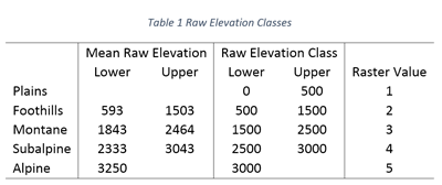
Two separate elevation classes were created. Both classifications systems were created based on a review of vegetation life zones (alpine, subalpine, montane, and foothills) in mountainous areas of North America. Data were most readily available for zones in the Western US. At least five regions were used to estimate elevations for each life zone. The raw elevation categories are roughly based on the mean values for the upper and lower bounds of each life zone.
Secondary variables were then derived from the DEM. These
included latitude-adjusted elevation, landform, and modified heat load index
(HLI).
Latitude-Adjusted Elevation
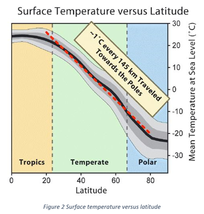
For regions north of the Tropic of Cancer, elevation was adjusted by latitude by adding ~1.14 meters for every 1-kilometer north of the tropics (23°N) (see Colwell et al. 2008). To convert the raw elevation values cited for each life zone into adjusted elevations, we estimated a latitude value (and consequently the # of kilometers north of 23°N) for each regional citation and then adjusted the elevation bands accordingly. We calculated the mean and standard deviation for the regional elevation breaks for each zone using the raw values and adjusted elevations using adjustment factors of 0.44, 1.14, and 1.8. The adjustment factor of 1.14 resulted in the smallest standard deviation and so seemed to be the most effective.
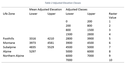
We based the adjusted-elevation categories on the mean of the adjusted breaks for each life zone (Table 2). However, while these breaks resolved elevation classes in mountainous western North America, the remainder of North America was essentially binned into the lowest (for the eastern and southern portions of North America) and the highest (for Alaska and much of the Arctic) bins. Therefore, we divided these bins (the lowest and the highest) into additional categories.
Click on the figure captions below to see high resolution images of the maps on this page.
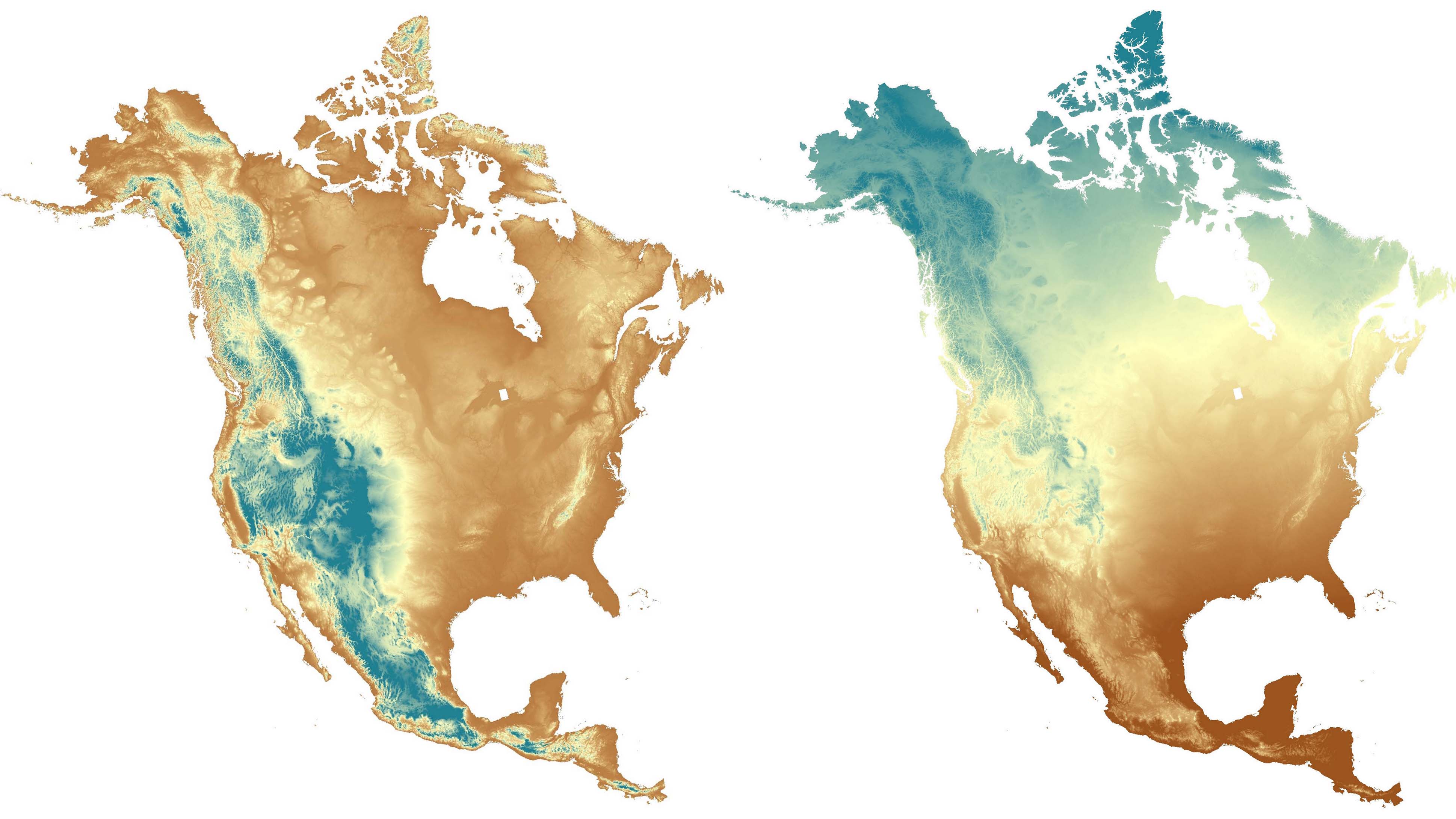
Figure 1. Non-adjusted elevation (a), latitude-adjusted elevation (b).
Landforms
Landforms were classified using a combination of Topographic Position Index (TPI) and slope based on the approach outlined in Jenness (2006). TPI is defined as the difference between the elevation of the focal cell and the mean elevation of the surrounding cells within a defined “neighborhood.” We created two TPI layers, one with a 2-kilometer moving window to identify large-scale regional topographic features such as mountains and valley canyons and another with a smaller 500-meter moving window to identify small-scale features such as headwaters, hilltops, and local ridges and valleys. We used a slope layer to distinguish between flat (< 2°), gentle (> 2° and < 5°) and steep slopes (> 5°) (Table 3).
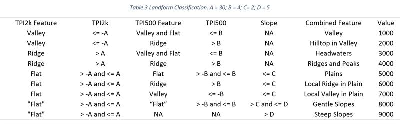
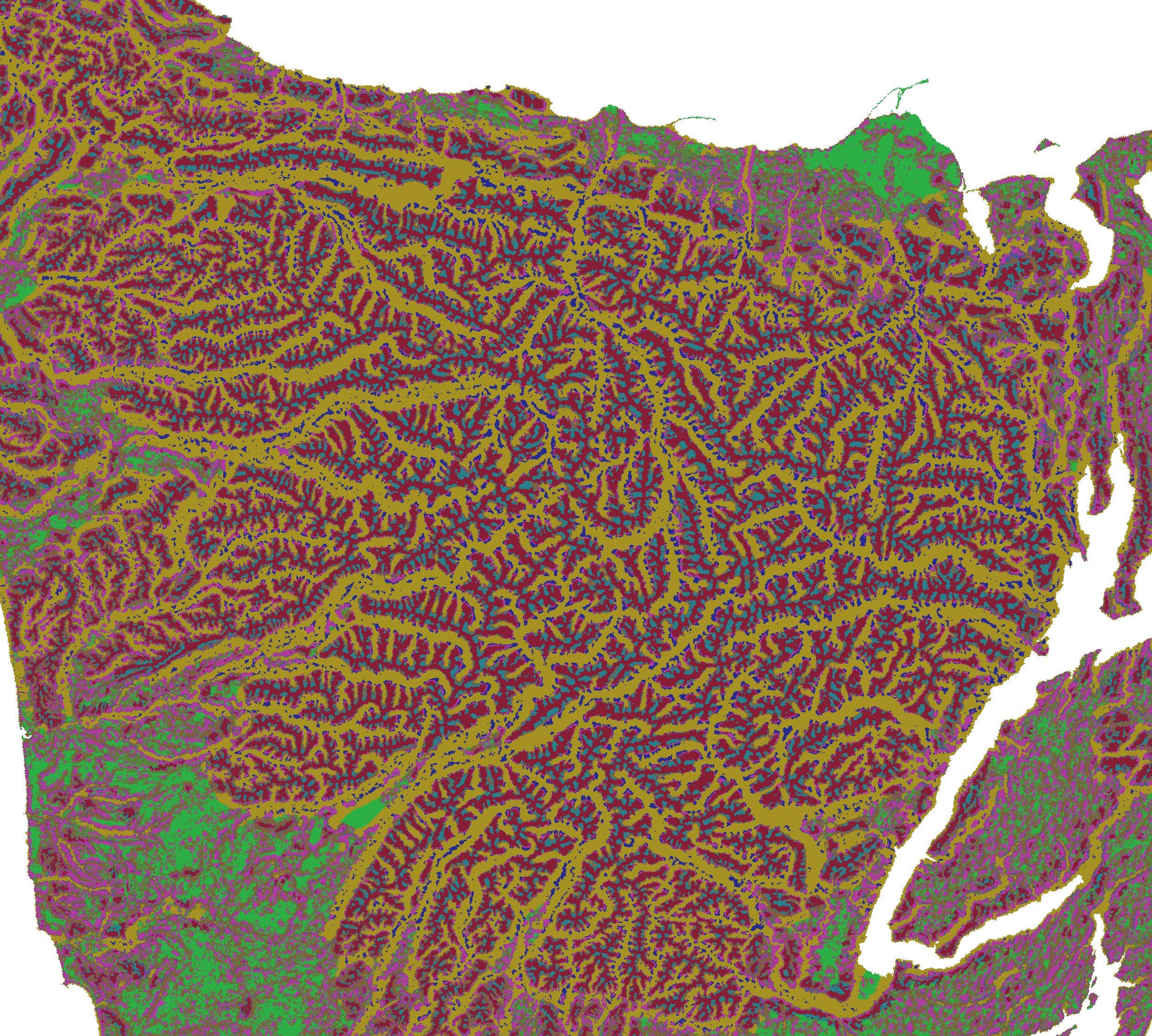
Figure 3 Landform classes for the Olympic Peninsula, Washington, USA.
Modified Heat Load
Index (HLI)
Heat load index (HLI) integrates aspect and slope to
quantify direct incident radiation and calculate a relative index of heat load.
It can therefore be used to identify relatively warm and cool areas of the
landscape with northeast slopes being coolest and southwest slopes being
warmest. We modified the heat load index
developed by McCune and Keon (2002) to remove the effect of latitude. In the
original index, latitude dominates over the influence of aspect and slope,
lessening the utility of the index for the purposes of defining physical
habitat types at a continental extent.
HLI is based on the relationship between insolation and aspect. One challenge with developing aspect data at a continental extent is that in commonly used projections, mapped north does not represent true north except along the central meridian. This distortion will be of greater importance in a continent-wide dataset than it would be in a regional dataset whose projection could be optimized for a smaller region. We addressed this by deriving aspect in a projection that maintains true north and reprojecting back into Lambert Azimuthal Equal Area projection (see this link for more information).
The HLI layer was divided into three categories: warm, neutral and cool. All cells defined as “Plains” in the landform category were by default classified as “neutral.” Remaining cells were classed into warm, neutral and cool depending on their HLI values. HLI values less than or equal to 0.223 were classed as “cool,” greater than 0.223 and less than or equal to 0.24 were “neutral,” and greater than 0.24 were “warm.” The break values were based roughly on the 33rd and 66th percentiles of HLI values for two relatively flat ecoregions, the Willamette Valley and the Columbia Plateau.
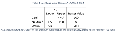
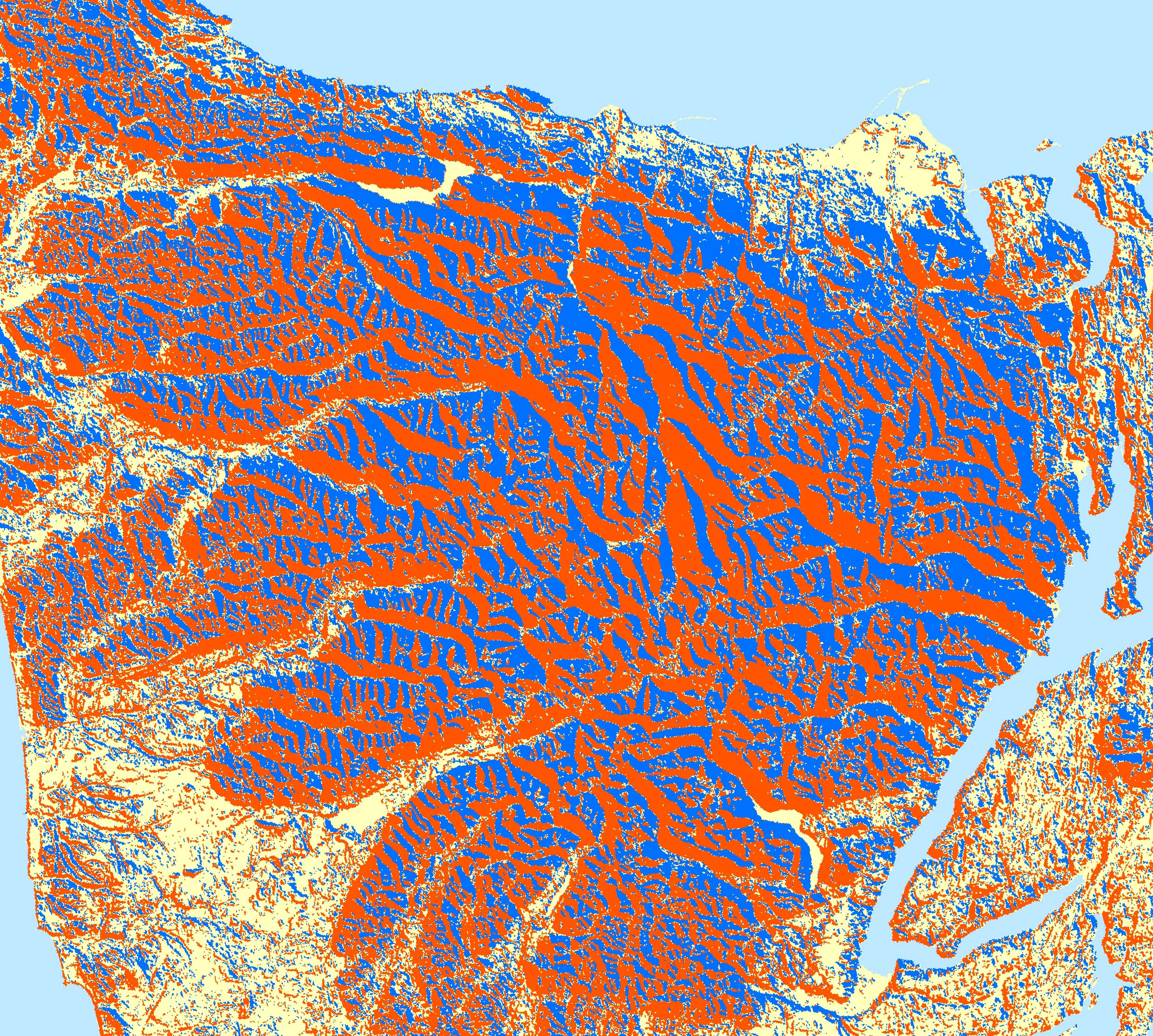
Figure 4. HLI classes for the Olympic Peninsula.
Soil order
We used the harmonized world soils dataset, which has a roughly 1-kilometer (30 arc-second) resolution and used soil orders to classify soil types. There are 38 soil orders. We were not able to use higher resolution soils data (e.g., STATSGO soils data for the US) because soil classes needed to be cross-walked across North America. We provide a topofacets data layer without soil order because the 1 km resolution of the soils data contrasts with the 100m resolution of the DEM-derived variables.
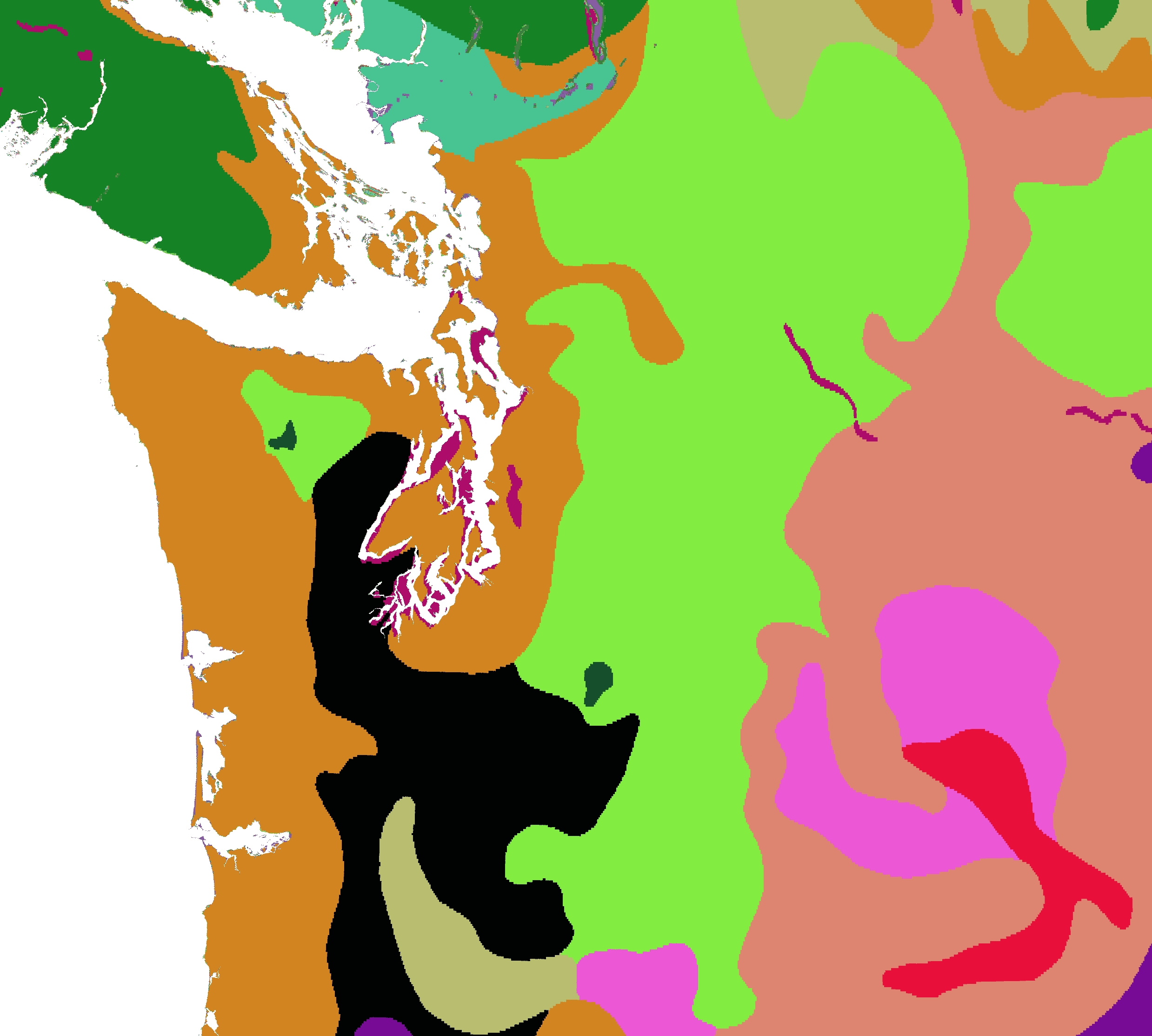
Figure 5. Soil order for the state of Washington, USA.
Once the continuous variables were categorized into discrete classes, the different categorical variables were combined into a composite land facet type. First, landform and HLI classes were combined into a composite type.
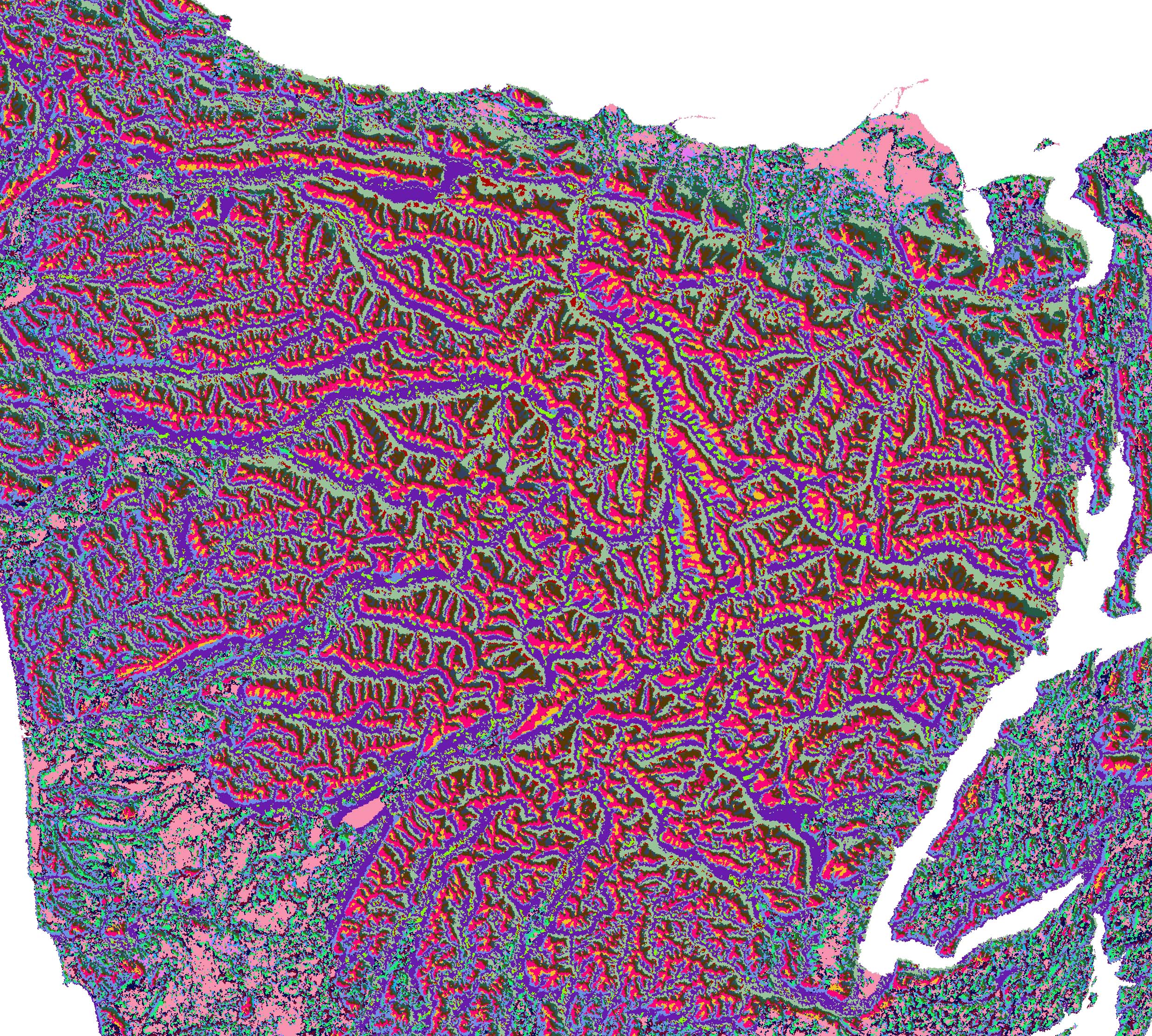
Figure 6. Landform-HLI classes for the Olympic Peninsula.
The resulting raster was combined
with elevation and soil type using the following system:
Facet ID Values = (Landform + HLI + Elevation)*100 + Soil Order
to create a final land facet type dataset. However,
because the global soil type dataset used here is of much lower resolution than
is the DEM, we also created a topofacet type
layer derived from HLI, landform, and elevation.
Topofacet ID Values = Landform + HLI + Elevation
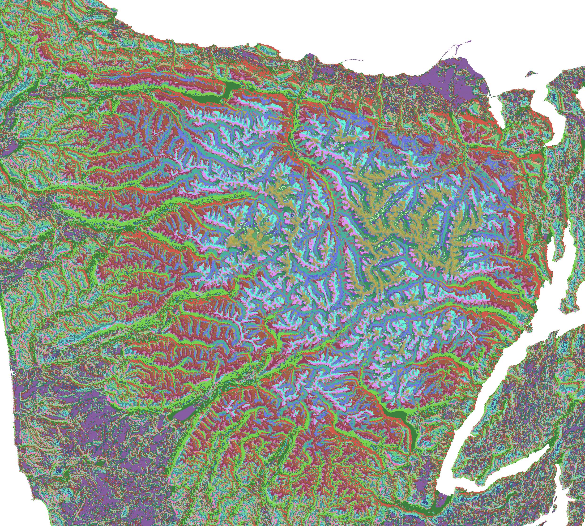
Figure 7. Topofacet classes for the Olympic Peninsula.

Figure 8. Topofacet (left) and land facet (right) classes for Washington state and North America.
There are many systems in use which categorize physical habitat variables into land facet types. Additionally, related efforts add ecological variables in order to categorize ecotypes. The data we developed are a useful representation of physical habitat at relatively high resolution and broad extent. Additionally, a USGS-led project has mapped ecotypes at 250m resolution at a global extent. A Nature Conservancy project has mapped enduring features across the northwestern USA. The ERGo dataset maps landform types for the contiguous US (Theobald et al. 2015). We will add links to other such datasets as they become available.
Download links for gridded data (100m resolution)
The gridded data available below were developed in a
Lambert Azimuthal Equal Area projection, at 100m resolution, and
covering North America.
The data is provided via a link to a
zipfile containing TIFF (.tif) format files that can be imported into
ArcGIS or other GIS applications. Please cite the
datasets below as:
Michalak, Julia L., Carroll, Carlos, Nielsen, Scott E., & Lawler, Joshua J. (2018). Land facet data for North America at 100m resolution. [Data set]. Zenodo. http://doi.org/10.5281/zenodo.1344637
The methodology used in producing the data is also described in the following citation:
Carroll C, Roberts DR, Michalak JL, et al. Scale-dependent complementarity of climatic velocity and environmental diversity for identifying priority areas for conservation under climate change. Glob Change Biol. 2017;23:4508–4520. https://doi.org/10.1111/gcb.13679
| Metric | Type of data used in metric | File size | Download link | |||
|---|---|---|---|---|---|---|
| Elevation | Heatload | Landform | Soils | |||
|
Land facets incorporating latitude-adjusted
elevation
|
X | X | X | X | 1GB |
|
|
Land facets incorporating non-adjusted elevation
|
X | X | X | X | 1GB |
|
|
Topofacets incorporating latitude-adjusted elevation
|
X | X | X | 1GB |
|
|
| Topofacets incorporating non-adjusted elevation | X | X | X | 1GB |
|
|
| Latitude-adjusted elevation categorized into 10 classes | X | 30MB |
|
|||
| Non-adjusted elevation categorized into 5 classes | X | 28MB |
|
|||
| Landforms categorized into 9 classes | X | 411MB |
|
|||
| Heat load index (HLI) categorized into 3 classes | X | 309MB |
|
|||
| Soil Order | X | 20MB |
|
|||