AdaptWest - A Climate Adaptation Conservation Planning Database for North America

Community

Meet…

Members

Groups

Data Basin Team

Join in…

Events

Become a Member

Donate

Workspace

Your workspace is your dashboard for accessing and managing your content, bookmarks, and groups, as well as viewing messages and seeing your recently viewed content.

You need to be signed in to access your workspace.

AdaptWest |
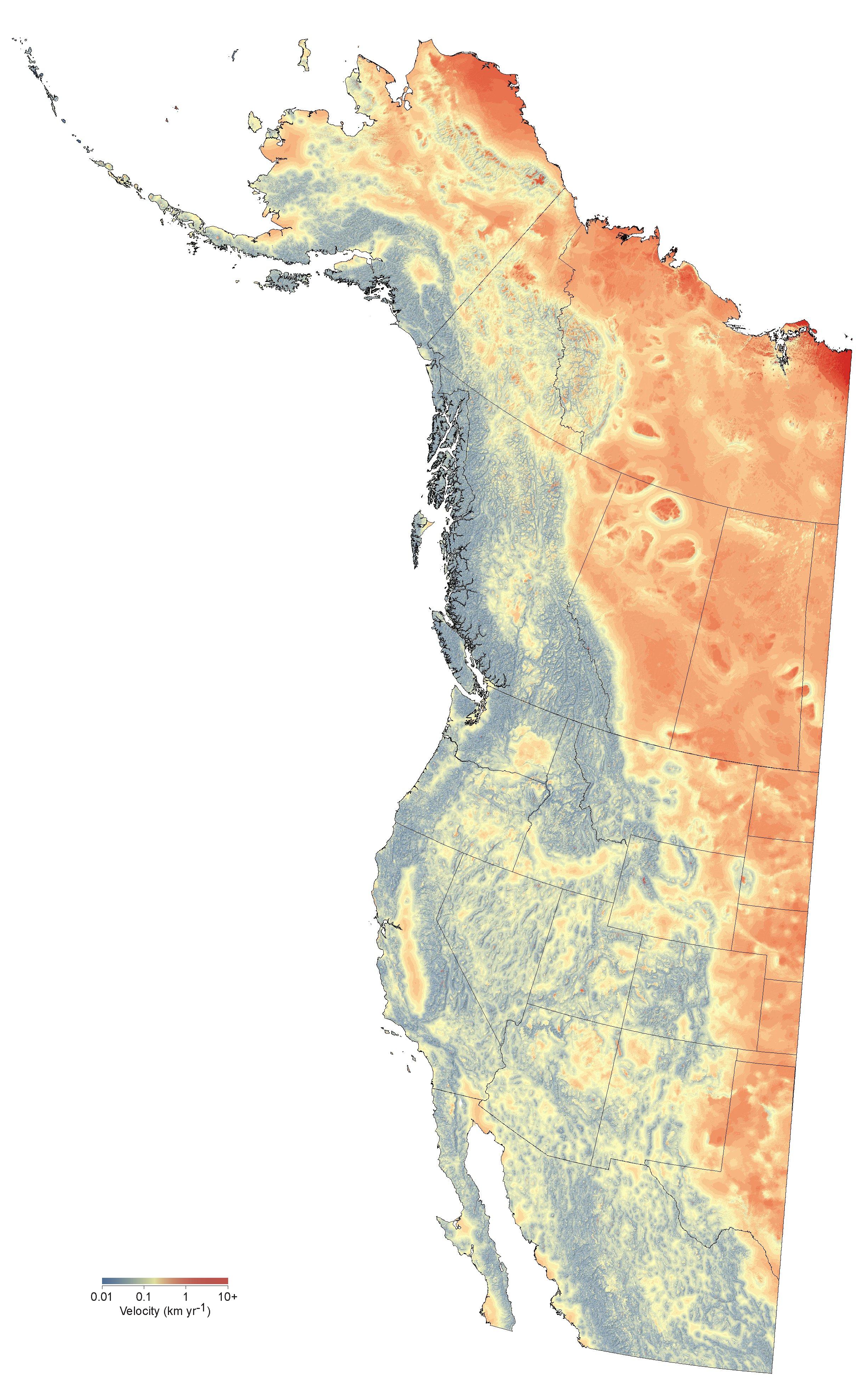
Velocity of climate change grids for western North America

Velocity of climate change grids for western North America

This dataset has been prepared for the Climate Adaptation Conservation Planning Database for Western North America (CACPD) project, funded by the Wilburforce Foundation with additional contributions from the GenomeCanada AdapTree project. It is based on Parameter Regression of Independent Slopes Model (PRISM) climate data for the 1961-1990 normal period (see http://tinyurl.com/ClimateWNA), and climate change projections of the Coupled Model Intercomparison Project phase 3 (CMIP3) database corresponding to the 4th IPCC Assessment Report for future projections.

The velocity of climate change is an elegant analytical concept that can be used to evaluate the exposure of organisms to climate change. In essence, one divides the rate of climate change by the rate of spatial climate variability to obtain a speed at which species must migrate over the surface of the earth to maintain constant climate conditions. Here, we provide data from an improved algorithm that conforms to standard velocity calculations if climate equivalents are nearby. Otherwise, the algorithm extends the search for climate refugia globally. Below we provide velocity surfaces for mean annual temperature (MAT) as well as a multivariate PCA implementation that searches for climate matches in 12 biologically relevant climate variables.

Futher we distinguish, forward and backward velocities allowing useful inferences about conservation of species (present-to-future velocities) and management of species populations (future-to-present velocities). For the forward calculation we ask: what is the rate at which an organism in the current landscape has to migrate to maintain constant climate conditions? Conversely, in the reverse calculation we ask: given the projected future climate habitat of a grid cell, what is the minimum rate of migration for an organism from equivalent climate conditions to colonize this climate habitat? For more information see:

Hamann, A. and Roberts, D.R., Barber, Q.E., Carroll, C. and Nielsen, S.E. 2014. Velocity of climate change algorithms for guiding conservation and management. Global Change Biology Pre-print on-line, DOI: 10.1111/gcb.12736.

Algorithms for generating velocity surfaces	Download
Sample data for algorithms below	ASCII:
Univariate, complete search, simplest algorithm	Word:
Univariate, complete search, faster algorithm	Word:
Univariate, kNN search, xy coordinates, fastest algorithm *	Word *:
Univariate, kNN search, smoothed grids	Word:
Multivariate, kNN search, xy coordinates, fastest algorithm	Word:
Multivariate, kNN search, smoothed grids	Word:

*) recommended code to get started. Default settings should work with any mean annual temperature grid.

Click on the thumbnails below and use the zoom tool

to see high resolution images of univariate and multivariate, forward and reverse climate change velocities for western North America

Download links for gridded data (1km resolution)

The gridded climate layers downloadable below are in Lambert Conformal Conic projection, at 1km resolution, and covering North America, west of 100° longitude. The database consists of ESRI grids, a native format of ArcGIS software, but compatible with many other GIS applications.

Type of velocity of climate change calculation	Emission scenario¹	Future period²	7 selected CMIP3 AOGCMs³	Average Ensemble Projection
Mean Annual Temperature, Forward (present to future)	A1B	2020s	ASCII:	ASCII:
Mean Annual Temperature, Forward (present to future)	A1B	2050s	ASCII:	ASCII:
Mean Annual Temperature, Forward (present to future)	A1B	2080s	ASCII:	ASCII:

Mean Annual Temperature, Reverse (future to present)	A1B	2020s	ASCII:	ASCII:
Mean Annual Temperature, Reverse (future to present)	A1B	2050s	ASCII:	ASCII:
Mean Annual Temperature, Reverse (future to present)	A1B	2080s	ASCII:	ASCII:

Multivariate, Forward (present to future)	A1B	2020s	ASCII:	ASCII:
Multivariate, Forward (present to future)	A1B	2050s	ASCII:	ASCII:
Multivariate, Forward (present to future)	A1B	2080s	ASCII:	ASCII:

Multivariate, Reverse (future to present)	A1B	2020s	ASCII:	ASCII:
Multivariate, Reverse (future to present)	A1B	2050s	ASCII:	ASCII:
Multivariate, Reverse (future to present)	A1B	2080s	ASCII:	ASCII:

   ¹) B1: low emssion scenario, A1B: moderate emission scenario, A2: high emssion scenario.
   ²) 2020s: average for years 2011-2040, 2050s: 2041-2070, 2080s: 2071-2100.
   ³) 7 AOGCMs selected based on the table and graph below.

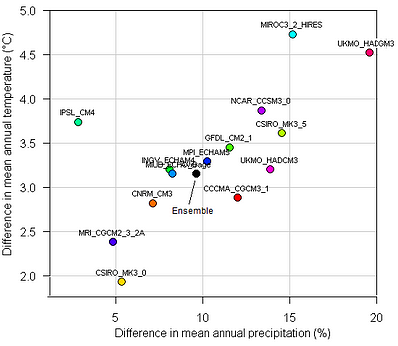
NOTE April 20, 2020: A minor downscaling error was found in a subset of the monthly and seasonal variables for HadGEM2-ES, and we have disabled download of velocity data based on this GCM until further notice.

AOGCMs

How to select future climate scenarios

Selecting scenarios for climate change impact and adaptation research is a complex task. Not all future projections have equal resolution, number of runs, and validation statistics against past climate. We selected a representative set of 7 AOGCMs from 14 high-quality models, from a total of 23 CMIP3 AOGCMs.

To further whittle the number of AOGCMs under consideration down, researchers often select "worst case", "best case", and "median" climate change projections. However, what constitutes a worst case or best case scenario, differs by region and by the climate variable of interest.

The plot on the right may help with scenario selection for the entire study area, and the table below for scenario selection for regions within western North America. We also provide ensemble scenarios for download above, but they may have unrealistic combinations of individual climate variables.

AOGCM_table